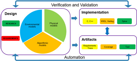
Chicken or egg, physical model or prototype hardware? Physical models are used in Model-Based Design to create closed loop simulations to validate control algorithms. To close the loop with confidence the physical model needs to be validated against the real world. And there is the rub; how do you validate a physical model when you may or may not have access to the hardware?
The real world, or something like it…

It is rare that a product is truly “new” and so we can often start off with an atlas(1) that provides initial directions. From there, validating the physical model takes the following series of steps
- Determine which variables influence your outputs
- Determine which of those variables can directly and safely(2) be measured
- Determine the accuracy of those measurements
- Determine the operating conditions of your model(3)
- Find the “boundary” effects, such as hard stops or friction / stiction interactions.
C3:(4) Collect, clean, correlate!

The first two C’s, collect and clean, are performed on the proto-type hardware or taken from existing research. Once collected, outlying data is discarded and the process of correlating the physical model to the real world data starts.
In an ideal world the inputs to the physical hardware can be directly fed to the physical model and the outputs compared. The model is then “tuned” to reach the highest level of correlation.
Building up from simpler models…

Sometimes the full physical device is not available for data collection. In this case your physical model architecture is built from correlated “submodules.” In this case the accuracy of calculations is even more critical. For the simple case where the accuracy is consistent across the full operating domain it can be calculated as
acc(tot) = acc(1) * acc(2) * … * acc(n)
However, since it is more common that the accuracy is dependent on where in the operating envelope you exercise the model it should be calculated as
acc(tot,r1) = acc(1,r1) * acc(2,r1) * … * acc(n,r1)
acc(tot,r2) = acc(1,r2) * acc(2,r2) * … * acc(n,r2)
acc(tot,rm) = acc(1,rm) * acc(2,rm) * … * acc(n,rm)
In operating regions where sub-models have lower accuracy it is important to maintain high levels of accuracy in the other sub-models.
Footnote
- This is both a reference to the image and a chance to say, image searches on the phrase “the real world” bring up the MTV show and almost nothing else.
- Remember, one of the reasons for physical models are to take the place of tests in unsafe operating conditions!
- Sometimes multiple models are required to handle different operating conditions.
- The “3” here was in the mathematical sense, C to the third power. The 4 in parenthesis is the footnote.


One thought on “First Principles of Physical Model Verification”