Part of my objective in writing this blog is to clarify issues that are seen as complex to render them to the “actual complexity of the system”; simplify without sacrificing accuracy. Recently when looking up information on transmissions I came across this video from Chevy from 1936, explaining how a transmission works. While modern transmissions have additional components not covered in this video (such as hydraulic clutches) the fundamentals are there.
With that in mind, today I want to take this opportunity to highlight another excellent work that explains a fundamental engineering concept.
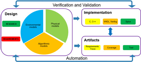
Selecting an ECU (electronic control unit) for your project is an investment in time and financial resources. Once the selection has been made for a given product line, that ECU will be used on average for 5 years. This means that even if the ECU meets all of your needs now it may not in 3 years if you don’t plan ahead.
Types of growth
There are three types of growth that need to be accounted for:
Increases in functions: as new features are added new functions are added. These functions will take up additional processing time.
Increases in memory: Hand-in-hand with the new functions’ time needs are memory needs.
Increases in I/O: The trickiest of the lot. Sometimes it is just additional channels of existing I/O types but in some cases it is a need for new I/O types.
As a general rule of thumb, 80% to 85% memory process utilization at initial release provides a safe margin. For hardware, two spare channels of each type is generally safe. In the case where new I/O types may be required there are two options. The first is to select a hardware device that has product family members with additional I/O types. The second is a selection of a board that supports external I/O expansion slots.
Growth in the times of DevOps
Traditionally the updates to ECU software only happened when a new product was released and it happened “in the factor.” With the growth in “over air” updates (one of the driving features of DevOps) the starting metrics need to change. The rule of thumb will need to take into account the anticipated features to be released and determine which of those will be pushed for update. The type of features to be pushed will be heavily dependent on the product type with some products receiving very few updates (e.g., medical devices with high integrity workflows) while others such as consumer devices may receive frequent updates
Simulink is a graphical control design environment. However, it has the ability to include MATLAB, textual-based, algorithms as part of the model. For some design problems, this is the best approach. In today’s post, I’m going to review the three primary methods for including MATLAB code in your Simulink Model.
Function / Class / System Object
There are three methods for including MATLAB code into Simulink Models; a function, MATLAB classes, or MATLAB Simulink System Objects.
Function
Class
System Obj
Generates C code
X
X
X
Simulate
X
X
X
Supports calls to external files
X
X
X
Object Oriented Code
X
X
Built-in I/O validation routines
X
Built-in state save / restore methods
X
Features Summary
The Class and System Objects provide functionality that is not built into the Function method. However, both require additional knowledge of how to program. A MATLAB function can be written as a simple set of equations while the Object Oriented methods require some base level programing knowlege.
And state data: memory
For models that are targeting Code Generation there is an additional consideration, memory usage. State data, or dWork data in the generated code is used for any variable that is required to be held in memory between time steps. With a MATLAB function the user can explicitly define the variables that are State Data by using the “persistent” keyword.
Example of calling a MATLAB class from within a MATLAB function block in Simulink
With the MATLAB class or MATLAB System Object, any data that is defined as a property will be stored as a dWork variable regardless of the need for a state variable. The number of state variables can be decreased in the Class implementation; however in doing so, much of the benefit of the class based approach is lost.
Co-Simulation is when two or more modeling tools run concurrently, exchanging data between the tools. Co-Simulation is desirable when a single tool cannot achieve either the fidelity or execution speed required to model a given element.
Types of co-simulation
There are two primary types of co-simulation: imported and networked.
Imported: The “primary” tool incorporates the “secondary” models into its’ framework. The primary tool is responsible for the execution and timing of the secondary tool.
Networked: In the networks, case the tools execute independently with a secondary program providing the data exchange layer between the tools. The data exchange layer is responsible for matching the time stamps for the tools.
Why Imported?
If your primary tool has a method for importing third party executables, like S-Functions in Simulink, then this is generally the easiest method for performing co-simulation. Once the functional interface is defined, the simulation engine of the primary tool provides the full execution context.
The downside of this approach is that it’s generally less accurate than the networked option. This is most acute when either of the tools requires a variable step solution as the incorporated tools are most often run at a fixed step or a variable step set by the primary tool.
Why Network?
In contrast, the networked approach allows you to run each tool with the optimal step size for the model; this results in high accuracy but is more often than not, much slower. The second issue with this approach is, how do you synchronize the tools?
In general a 2nd or 3rd order spline should be used to match the data points between the tools for the different time steps. This means that the integration tool may need to store large amounts of data and perform significant calculations at each data exchange.
There are some texts that serve as a foundation stone for a field or technology; Kernighan & Ritchie’s “The C programing language” for C, Smith, Prabhu and Friedman’s “Establishing A Model-Based Design Culture” for MBD and for UML it is Martin Fowler’s “UML Distilled.” While the fields have moved beyond these three texts they all act as the common starting point of the discussion. With that in mind I want to talk about why reading UML Distilled will provide a significant boost to your system level modeling abilities.(1)
The third, and latest addition of UML Distilled was written in 2003. The usage of UML and the associated tool chains have evolved since then but the core principals of the book hold up.
A definition that holds up to the test of time
The difficulty in talking about UML is that it is an open standard; as a result, different tools and different groups have variants on the implementation of the language. That is why this book is so valuable, it lays out the core nature of the major types of UML diagrams.
When to use!
Perhaps most importantly the book lays out the cases of when to use each type of UML diagram, e.g. “Class Diagrams: When to use” & “Sequence Diagrams: When to use” and… While in my view the book recommends the usage of some diagrams when I do not think the are appropriate (specifically some of the recommendations for State Machine Diagrams and Communication Diagrams) it is admirable that he provides the trade-offs between different types of UML diagrams.
Object Oriented Classes and UML
One of the virtues of UML is the ability to graphically design Object Oriented models using Class Diagrams. Combined with Sequence Diagrams, the basics of a systems level modeling tool can be defined. However, what is often missed is that the Class and Sequence diagrams need to be combined with Package and Deployment diagrams to fully implement a system level model. Often the first two are used in system design and a less efficient implementation is created.(2)
Footnotes
The primary issue surrounding UML is “when to stop.” UML diagrams are not intended for the final design of software but it is tempting to keep putting more information into the UML diagram. Fowler lays out a good case for how far to go.
For smaller systems, Class and Sequence diagrams are sufficient; however, for larger system-of-systems the Package and Deployment diagrams are needed.
The early promise of “Internet of Things” (IOT) offered refrigerators that would let us know when to buy more milk/ But the reality often failed the C3 test,(1) being more hype than help. However, with the growth of big data analysis IOT has come into its own.
Who is IOT for?
By its nature IOT is collecting data on the end user. For consumer goods this can be an invasion of privacy; for industrial goods this can be violation of production secrets. So the answer to “who is IOT for?” needs to be “for the customer.”
Predictive maintenance and IOT
I remember when I was 16 pulling into a friend’s driveway. His father who was in the garage looked up and said to me “your timing belt is going to break in about 5,000 miles.”(2) He knew it by the sound and he knew it by the data he had collected and analyzed. When a product ships, the designers know a subset of what they will know two, three, a dozen years in the future. IOT allows them to learn what the failure modes for the device are and then rollout those failure modes to the end user.
IOT and MBD
Model-Based Design needs to interface with IOT in two ways. What to upload and how to update. As part of the design process engineers now need to think about:
What data would be useful to improve performance?
What is the frequency of the data collection?
How much memory do I allocate for storing that data?
Put another way, your IOT strategy is the feeder to your DevOPs workflows.
Footnotes
The C3 test, or “Chocolate Chip Cookie” test is when an operation is linear then a simple algorithm can determine when to order the next 1/2 gallon of milk. However, some things like getting chocolate chip cookies which require “milk for dunking” break the linear prediction (unless you have them all the time).
I had some great questions from the “Reader request” post. Today I will set about answering the first batch, the hardware questions.
Why is hardware hard? Does it need to be?
There were a set of questions connected to targeting specific hardware, e.g. how to generate the most efficient code for your hardware. Within the MATLAB / Simulink tool chain there are 3 primary tasks:
Configuring the target board
The first step is to configure the target hardware through the hardware configuration menu. This defines the word size and ending nature of the target hardware.
Calling hardware devices
MATLAB and Simulink are not designed for the development of low level device drivers for physical hardware. However they are wonderful environments for integrating through defined API’s calls to physical hardware. The recommended best practice is to create interface blocks, often masked to configure the call to the API, which route the signal from the Simulink model to the low level device driver
Speedgoat Interface block
Another best practice is to separate the IO blocks from the algorithmic code, e.g. create Input Subsystems and Output Subsystems. This allows for simulation without the need to “dummy” or “stub” out the IO blocks.
Make it go fast!
The final topic is deeper than the scope of this project; how to optimize the generated code. Assuming an appropriate configuration set has been selected the next step is to use board specific libraries. Hardware vendors often create highly optimized algorithms for a subset of their mathematical functionality. Embedded Coder can leverage those libraries though the Code Replacement utilities. One thing of note, if this approach is taken then a PIL test should be performed to verify that the simulated behavior of the mathematical operation and the replacement library are a match.