Model-Based Design: Projects of interest

Early in my career one of my mentors made the statement

“If we understand the system we can model it.
If we can model it we can make predictions.
If we can make predictions we can make improvements”

In the past 20+ years, I have not heard a better statement of the driving ethos behind Model-Based Design.

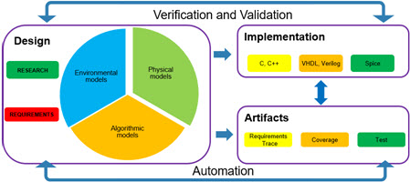
If we understand the system, we can model it:(What we need to do): when the system is understood, it can be described mathematically.  This could be a derived first principal model or a statistical model; the important thing is that the confidence in the model fidelity is understood.

If we can model, we can make predictions:(What we can do): once the model is known it can be used.  The use of the model can be in the design of a controller, predicting a rainfall or embedded within a system to allow the system to respond with better insight.

If we can make predictions, we can make improvements:(Why we do it): this last part is the heart of Model-Based Design.  Once we can make accurate predictions we can use that information to improve what we are doing.

Model and equation…

Models build on a foundation of equationsflightdynamics to provide a dynamic, time variant representation of the real-world phenomenon.  Moreover those equations are working as part of a system; you leverage models when you move into complex systems with multiple interdependent equations.  Within the Model-Based Design world, we most often think of these systems as closed loop system.  Similar examples can be seen in the social sciences, in biology and chemistry.

Understanding from a sewage treatment plant…

Coming from an aerospace background, and starting my working career out in the automotive industry the general nature of models sunk in during one of my earliest consulting engagement; helping a customer model a sewage treatment plant to determine optimal processing steps against a set of formal requirements.

  • Requirements
    • The plant may not discharge more than N% of water in untreated state
    • The plant’s physical size cannot exceed Y square miles
  •  Objectives
    • Minimize the total processing cost of sewage treatment (weight: ω)
    • Minimize the total processing time of sewage (weight: λ)
    • Maximize the production of  energy from bio-gas (weight: Φ)
    • ….
  • Variants of inputs
    • Sewage inflow base rate has +/- 15% flow rate change
    • Extreme storm conditions can increase flow rate by 50%
    • ….

The final system model included bio-chemical reactions, fluid dynamic models, statistical “flush rates” and many other domains that I have now forgotten.  The final model was not able to answer all of the questions that the engineers had, however, it did allow them to design a plant with significantly lower untreated discharge rates and lower sewage processing costs.  This was possible because of the models.  This was the project that showed me just how expensive Model-Based Design is.

Initial adoption: objectives and metrics

Objectives and metrics

Based on the information collected from the process adoption team the objectives for the initial adoption phase should be set.  While the specifics for any given organization will be different the following outline is a standard view.

1403204517-3-keys-measure-success-loyalty-program

  1. Technical 
    1. Complete 1 or 2 “trial” models
      1. Identify the initial model architecture
      2. Identify the initial data architecture
      3. Establish baseline analysis methods
      4. Establish baseline testing methods
    2. Understand how artifacts from models integrate with existing artifacts
    3. Implement version control for new modeling artifacts
  2. Managerial
    1. Review methods for measuring model key performance indicators (KPIs)
    2. Review resources required during initial adoption phase

The technical metrics

Completion of the trial models

In a future post we will examine how to select your trial model,  but for now let’s answer the question “what does it mean to complete a trial model? ”  This decomposes into the four tasks as outlined above.  The model and data architecture are covered in some depth in previous posts so let us talk about analysis and testing.

Within the Simulink domain, a fundamental aspect of a model is the ability to simulate the behavior of the plant or the control algorithm. analog-simulationThe simulation is used during the early stage of development to analyze the model to determine if the functional behavior of the model.  The developer performs elaborates the model until the behavior functionality matches the requirements.  This is verified through simulation.  Once the model meets the requirements the functionality can be “locked down” through the use of formal tests; again using simulation.

It is worth noting that some requirements will be met before others, they should be formally locked down under test as they are achieved.

Integration with existing artifacts

For most companies, unless they are starting from
integratesoftwarea clean sheet there will be existing software components that need to be integrated with those created by the Model-Based Design process.  There are three types of integration

  1. bringing existing software into the Model-Based Design framework
  2. Bringing Model-Based Design artifacts into the existing architecture.
  3. A combination of 1 and 2.

The topic of integration will be covered in greater detail in an upcoming post.  However, the fundamental guidelines for integration (in either direction) are the following.

  • Create software objects with well-defined interfaces (encapsulation)
  • Limit dependencies of the software objects on external objects
  • Minimize the use of “glue code”(1).

Version control of objects

Version control processes use tools to enable team-based development while maintaining multiple “release” or “branches”.  During the initial phase of the project which software objects will be placed under control and how a “release” will be defined should defined.  This initial definition will be refined as the Model-Based Design process is elaborated.  This blog will go into detail on this in a future post.  The basic questions are

  • Do you include derived objects in the version control software: .c, .h, test reports…
  • How do you arbitrate check in conflictsHow do engineers resolve conflicts in their model interfaces?
  • How do you share data / models across projects: What methodology will facilitate reuse of objects across multiple projects with minimal configuration impact?

Managerial metrics

The initial adoption phase by its nature will be slower than later phases as people are still learning new capabilities and processes.  57572027-gears-and-kpi-key-performance-ind-cator-mechanismThe primary objectives during this phase are

  1. Learn what bottlenecks with the new process.
  2. Understand existing issues uncovered by the transition
  3. Determine level of resources for the next stage

The discovery of “Objective 2’s”, existing issues, often surprises people.  The act of transitioning to a new process forces the evaluation of existing processes and, more often than not, illuminates existing shortcomings.  Extra care should be taken to ensure that the new process addresses those shortcomings.

In the next stage, the validation project, the team should expand beyond the initial “core” team. Ideally, a people from outside the initial project scope should be brought in to identify developmental pain points that did not exist in the “core group” processes.

Footnotes

(1): “Glue code” is a software object created solely for the connection of two other software objects.

Fidelity of plant models in closed loop simulation

In graduate school I studied computational fluid dynamics (C.F.D) as part of an aerospace engineering degree.  Understandably I was quite excited when my professional assignment was developing a throttle body model for GM’s hardware in the loop system (HIL). Making several assumptions and ignoring the boundary layer conditions I efficiently implemented a 2-d version of the Navier-Stokes equation:

stoked

The model accurately predicted the intake manifold pressure within 0.01% of the measured pressure at a time step of 0.002 seconds.  It used 45% of the HILs processing power (this was in 1995)

Plants in the Field

treeinfield

In the end, I derived a transfer function that modeled the system with 1% accuracy at the same time step using less than 1% of the processor.  That experience, and many since, have caused me to consider the question “what do you need from your plant model?” I have developed 4 basic questions I ask myself and my customers.

What is the required accuracy?

whycantyoudraw_3-2_look_at_things

What is the required accuracy?  In my example above the plant model was connected to a ECU through a 7 bit A/D.  The pressure range was from 1.2 ATM to 0.5 ATM, meaning a resolution of 532 mmHg / 128 = 4.15 mmHg was the best the sensor could do. Therefore from the controllers perspective, anything better than that was not required.  However, the plant model required an accuracy of 0.1 mmHg to maintain stability; a factor of 41 times greater accuracy than required.

There is a second component to accuracy, which is accuracy at the edge points.  A simple polynomial equation could be used to accurately model the throttle body during steady state operation; however during transitions that polynomials accuracy was no better than 10%.

Another example is an engine torque model.  A simple table lookup will provide the engine output torque over the nominal operating range of 800 ~ 5000 rpm.  However, engines do operate outside of that range; the fidelity with which you model those conditions is dependent on what you are validating within your system.

What are my resources?

There are two resources for computations, memory and calculation time (FLOPS for example).  In the example above the accuracy was much greater than required so we considered alternative methods.

The proposed alternative was a 2-D lookup table using two points of past data.  The calculations for the table look up took roughly half the FLOPS of the transfer function and the accuracy was in line with the requirements (1 mmHg).  However, the amount of memory required for the table was approximately 10 times larger than the transfer function(1).

In the end the much higher memory requirements prompted the selection to the transfer function as the solution.

Do you require multiple versions of the plant?

So far in this post, I have talked about targeting a HIL system.  However, it is often the case that a plant may need to be modeled for multiple domains.(2).  In that case developing interfaces to the plant that can be used across multiple environments is an important.  It is now common practice to embed model variants within a closed system to select which version of the plant is required depending

How much do you know about the plant?

The last question to ask in developing a plant model is what is known about the actual plant to enable validation of the plant model.  In some cases, where the physical plant does not yet exist first principal modeling must be done.Even in that, it is often possible to design part of the model based on previous similar plants.  This can be done through the parameterization of the plant model.

Footnotes

(1) In this example, the table data would have only been used by a single function.  If the same table data could have been used across multiple functions then a different decision may have been made.
(2) In a happy ending to my Navier-Stokes model was eventually used as part of another project

Understanding data usage in Model-Based Design Part II

In the last post we looked at the characteristics of data now we will at how those characteristics define and support the model.

Data defines the model behavior

Let’s imagine a model “estimate time to debug software.”  The first thing we could consider is the following simple mathematical model

bugsFound =3 * exp(timeCoef * T) dT
where: T = [0 : 7.5] (half hour lunch break)
timeCoef = [-0.1 : 0.2]

And consider two parameter sets

  • Bored test engineer: timeCoef = -0.1
    • Bugs found in 7.5 hours: 15
  • Engaged test engineer: timeCoef = 0.1
    • Bugs found in 7.5 hours: 52

bugsfound

With this simple example, we see that changes to data affect the results of the model (equation).  In the actual model, we see multiple parameters associated with the “engaged” and “bored” test engineers.

Parameter Comment
BugsPerLine Common
LinesPerHour Engaged > Bored
GramCoffeePerHour Engaged < Bored
TimeAllocatedToFindBugs Commom

In a system level model, comprised of multiple integration models, there are multiple parameter sets.

plantmodel
Closed loop vehicle control algorithm and plant model

In this example, we have two top-level integration models, the controller, and the vehicle plant model.  Within those integration models, there are multiple parameter sets

  • Engine
    • number of cylinder
      • 8 cylinder
      • 6 cylinder
      • 4 cylinder
    • Throttle body
      • Standard
      • Turbocharger
      • Supercharger
  • Transmission
    • ….
  • Drive line
    • …..

Next steps

As this post shows the amount of data consumed by a set of models quickly grows in complexity.  In an upcoming post, we will look at best practices for data management.

Understanding data usage in Model-Based Design Part I

What is data and how is it used in a model centered development process?  We start by talking about different types of data.

Types of data

  • Algorithmic data:  data that is used or created by the algorithms.
    • Constants:  data values that are used in calculations that are fixed; for example, pi.
    • Parameters: data values that are used in calculations but can be tuned, or c by the engineer; for example a gain value for a PID controller.
    • Calculated values (signals): signals are the result of the calculations in the system
    • State: state data is a special case of signal data, it is the calculated data from previous time steps
      howfullami
  • System specification data: data that configures the system
    • Configuration:  Unique to Model Based Design configuration data specifies some of the base functionality of the models calculations.  This includes things such as integration methods, sample times, and code formatting.
    • Instance specification: meta data that specifies which set of algorithmic data is used to instantiate a given instance of the model(1).
    • Variant: data that configures which blocks of code execute; these are distinct from execution control as they are either compile time or start up controlled.  For example compiler #define options.
  • Verification and validation data: data that is used or created by the models and system for testing.
    • Input data:  inputs to the system used to drive the tests
    • Expected outputs: results based on inputs and the test configuration
    • Test configuration: data that configures the model (through selection of algorithmic and system specification data) for an instance of a given test.

Data attributes

All data has attributes that define how that data is interpreted by the system(2).  Some modeling environment explicitly exposes all attributes (Simulink, UML) while others (C, C++)  require users to have an external database to associate attributes.

Let’s focus on the attributes that all modeling languages share in common for algorithmic data; they are

  • Data type:  double, single, int, struct, enum…
  • Dimension: scalar, vector, matrix…
  • Storage class: Where the data is instantiated

percentofcake

Ideally, within the development workflow the attributes, such as minimum and maximum values, are used by verification and validation tools to ensure the correct behavior of the model.

Next post

In the next post I will look at how the data is used to configure models and model behavior.

Footnotes

(1) The initial values of the state data may be included in this configuration set.  Initial values for state data is a subset of the parameter data.
(2) The specific attributes for a given class of data will differ.

Modeling architecture with room to grow

In the last post we looked at the characteristics and objectives of modeling architecture.  In this post, we will look at one method for satisfying those requirements.

Shell games, the parent and child relationship

A system level model is built from multiple levels of integration models.

  • Functional (child) model: A model that is comprised of function code, e.g. a plant or control model.
  • Integration (parent) model: A model that built from multiple functional models.  The integration model does not have functional code but may contain execution order (scheduling) elements.

shellmodelint

In this example, there are three functional (child) models; their interface is defined through the use of “ports” and have the descriptive names of “Known_#” and “BUS_#”.  We will look at this convention more in the next section.

shellmodelfunct

The first iteration of the functional (child) model is what is known as a “shell” model.  The inputs and outputs of the shell model should match the defined interface, e.g. the data type (double, int, float or structure) and dimension (scalar, vector).  Further the outputs from the shell model should provide values that are “safe” for other functional components in the system(1)   As the shell model is elaborated the outputs will reflect the actual executable code.

System architecture with unknown interfaces…

For well-established systems the input and outputs from the system will be known ahead of time.  However, for newer projects, the functional interface may not be fully defined.  In this instance buses(2) can be used to provide a flexible interface.  Members of the bus are selected inside of the child model, because of this members can be added to the bus as needed without breaking the interface of other child models.

Rational behind this approach

This approach to developing the system level model has multiple advantages…

  1. First, it allows independent development of the functional models.  Engineers are free to develop their model as long as they maintain the functional interface(3).
  2. Unit level testing can start with the initial shell model
  3. This approach allows system level testing at an early stage of development.
  4. This system promotes reuse of components.

Limitations of this approach

Following this approach can lead to inefficient or unclear function interfaces if the engineers keep adding new things into the input and output buses.  This can be avoided by follow through periodic reviews of the interfaces.  I will cover rules for data management in future posts(4).

Footnotes

(1)In this example I show simple constant blocks.  More complex data can be outputs can be created using signal generator blocks.
(2) In the MATLAB / Simulink environment, a bus maps to a C structure.  The bus is members are defined as part of the data dictionary then the model can create instances of the bus.
(3) The reality of development is that at some point in time the functional interface will need to change; a change process should be put into place to account for the change to the bus definition or ports of the system.
(4) As a general rule of thumb buses (structures) should not be more than 2 levels deep (e.g. Structure in Structure) and each root level should have no more than 12 signals. Going beyond this can result in difficult to parse data structures.

Modeling architecture: Fundamentals

In this section, we start our discussion around software architecture.  Taking a broad perspective all software architecture has three attributes

  • Components: Components are the fundamental building blocks of all software; they contain the “guts” that enable the software to perform their required functions.  These could be viewed as functions or classes in C/C++ or models in the Simulink environment.
  • Connectivity:  Connectivity is how components exchange information (data) with other components.  For example, a function definition in C / C++ or input and output ports in a Simulink model
  • Scheduling and execution control: The software architecture allows for (and maybe) the entity that controls the execution of the components.  Note: this is not addressing the low-level O/S scheduling.

aid47662-728px-write-an-educational-objective-step-8

So knowing the attributes the next question is “what are the functional objectives?”

  1. Facilitates group and individual development workflows:  Individuals should be able to work on the component they are developing with minimal impact/reliance on other people in their group.  At the same time, the group should be able to use components from others at an early stage in development.
  2. Provides easy integration of components: The components should be able to easily “connect” with components in both the new model based environment and any existing text based (C) environment.
  3. Enables unit and system level testing:  Components should be designed with clearly defined external dependencies and they should be minimized.  At the system level, child models should enable testing early in the design process using shell models.
  4. Promotes reuse of components: Developers should be able to reuse components either directly or through some data-driven modification.
  5. Is efficient in both execution speed and memory usage:  The decomposition of the system level model into components should balance clarity with efficiency.

The final consideration is stylistic(1), how do you create a model architecture and components that are easy for controls, system and test engineers to understand?  The M.A.A.B. Style Guidelines provide a solid foundation for developing understandable components. In my next blog post, I will start looking at how components fit into system level architectures and how they can be elaborated and tested throughout the development cycle.

Footnotes

(1) While I list the final consideration as “stylistic” it is of the highest importance. As clarity of communication is essential for ensuring reuse (objective 4), ease of integration (objective 2) and allowing group and individual workflows (objective 1).

Adoption Time Line: Exploration Phase Part II

Continuing from an earlier post we now look at how you set the objectives for the initial adoption phase.

We need the champions

Before we proceed in setting objectives we need to talk about resources.  There are 3 resources that are required for an adoption process to succeed; they are

  1. Champions:  Technical and managerial support for the adoption process.  Without active advocates change will not happen.
  2. Time:  The champions need to have time allocated to working on the process change.  Ideally the technical champions will have 100% of their effort allocated to the adoption of the new process.  When the resources are allocated at less then 80% the change is likely to fail.
  3. Experience:  The people working on the project need to understand the current workflow so they can address its short comings and speak to the people outside of the adoption group.

An earlier blog post from LinkedIn provides additional details.

Setting goals

Based on the information collected from the process adoption team the objectives for the initial adoption phase should be set.  While the specifics for any given organization will be different the following outline is a fairly standard point

  1. Prior to start of initial adoption phase
    1. Allocate resources to the process adoption team in support of project
    2. Process adoption team completes identified required training
    3. Review reference materials to understand current industry best practices
  2. By completion  of initial adoption phase (1)
    1. Technical 
      1. Understand how artifacts from models integrate with existing artifacts
      2. Establish baseline testing activities
      3. Implement version control for new modeling artifacts
      4. Identify initial model and data architecture
    2. Managerial
      1. Review methods for measuring model key performance indicators (KPIs)
      2. Review resources required during initial adoption phase (2)

Bounding the problem

A word of caution; model-based design offers multiple tools and methods as part of the development workflow.  A common pitfall when establishing any new process is to “overreach” utilizing multiple new tools all at once, the resulting diluting of attention introduces errors of misunderstanding and results in a slower adoption of the process.  In the initial adoption phase posts, I will discuss the normal building blocks for Model-Based Design.

Next post

The next series of posts will cover model architecture and data management.  These topics will help in understanding the next phases of the adoption and establishment processes.

Footnotes

(1) The term “adoption” reflects the fact that there are existing resources to guide companies in adopting workflows.  I always encourage people to leverage existing information rather than creating new workflows from whole cloth.  This is critically important when working in a safety critical environment.
(2) Identifying the resources required for future phases should be based on the KPI information gathered from the initial adoption phase.  It should also take into account the “cost of learning” associated with starting a new process.

State Machine / Flow Chart

Image credit: XKCD.com

This post is an interlude from the mainline discussion of Model-Based Design.  Today I will discuss the differences between flow charts and state machines.  The most fundamental difference between the two is that a state machine has knowledge of the past based on its current state(s).

southernsnowproblem

The southern snow problem

To give an example, if you live, or have lived, in the southern part of the United States you are aware of the syndrome known as  snow panic.     The south can be an pleasant place in the winter filled mild walk able days (see left hand state “EverythingIsFine”) but once snow is predicted they enter into the right hand state “OhMyGodSnow” and huddle up “SafeAtHome” until either the snow is gone or food runs out.  All of this logic is captured in 4 states and can be evaluated in a with a maximum of 2 operations [(noSnow==FALSE)&&(food<=deltaFood)].

southernsnowproblemflow

By contrast the flow chart version of this has a average of three operations and manually maintains a state (wasInSnow).

But how does it scale….

When I first learned C programming my instructor provided the rule of thumb “Never nest If/Then/Else statements more than 3 deep.”  That rule of thumb still holds for State Charts (MAAB: NA_0038) and ladder logic .  Fortunately both can be “nested” in logical containers known as Subcharts.  Recommendations for when to sub-chart can be found here,MAAB: NA_0040.

So which do I use?

Like most engineering questions the answer is “the correct one.”  Remember the way to tell which is correct is ask yourself, do past states matter, then a state chart may be the way to go.  If everything is based on current information then use flow chart logic.  In the end favor clarity over dogma.

itisatrapflowchart

Next post:

In the next post I will return to adoption time line: exploration phase part II.