Month: March 2019

In 1999 the movie The Matrix introduced (2) millions of people to the philosophical question “how do we know if we live in the real world or a simulation”. As an engineer, working for a company that makes the “Matrix Laboratory” I have been thought about this idea and it’s logical extension; can we trick a machine into thinking it is in the real world?

Is this the real life? (3)

Simulations of reality have existed for a long time, from wind tunes, to lumped mass model to complex finite element models; they have been the backbone of engineering design. As powerful as these models have been they have been limited as simulations of physical properties, or perhaps a system of physical properties. The next generation of simulations attempts to simulate the complex nature of the real world, that is to say people and their semi-predictable behavior.

Humans as lumpy-mass models

Ok, first I’m going to need to write a lot of text here to make it all the way down this comic strip…

The world is filled with humans, roughly 7.6 billion as of the writing of this post. We are out there driving cars, walking in the street, making phone calls, cooking dinner, talking about philosophy and sitcoms. We do a lot of different things. When moving in a mass we are largely predictable; that is to say if you asked me to calculate how long it would take for 100,000 people to exit University of Michigan’s football stadium, I could give you an reasonable accurate answer for the total. If, however you asked me how long for a given person, well then it becomes more difficult. It is the aggregate behavior that is predictable. The issue is that for controllers that interact with the real world the aggregate is not enough.

So how do you go about simulating a pod of people? There are several basic methods.

• Conway’s game of life: “humans” can be simulated by giving them a set of basic “rules”. Those rules (with weighted objective functions) determine how they operate. Note: your rules here can’t be too perfect, real humans make mistakes. (Note this is often done using cellular automation approach)
• Genetic algorithms: The humans can be derived using genetic algorithms(5). In this case a set of baseline behaviors are defined as well as “mutations” or permutations on those behaviors.
• Fluid dynamic analogies: Fluid dynamic models do a good job with modeling flow “restrictions” around doors and changing widths of the system.
• Real world data (human in the loop): The most difficult to set up, but done well, mining the real-world for data on how people act, and react, provides the most accurate models. The previous three suggestions can be considered reduced form version of the “RWD-HIL”

Why do we want a matrix for our machine?

It is oft repeated question for self-driving cars, what happens if a child darts out in front of it? Because it is repeated so often it is now tested for heavily. But what about all the other things kids (or adults) do that are foolish? Ever drop something in the street and stop to pick it up? Every order a 100 tee-shirts instead of 1? Pull up on the throttle when you should have pushed down? In the end people are semi-random creatures. Creating realistic models of people allows us to create better control algorithms.

Footnotes

1. The image of the “red pill” / “blue pill” should not be taken as an endorsement of A/B testing as the only validation methodology
2. Note, it introduced people to the question, it does not mean that many people put much thought into it beyond “dude, how can you know?”
3. Note, if we do it correctly we never have to sing “mamma, my controller just killed a man”
4. A pod of people is of course a reference to “pod-people“; e.g. close enough to fool some people
5. Real people are created from generic algorithms so this should wok right?

If you find benefit from this blog, consider subscribing

In my last post, Execution order and Simulink models, I promised a look at scheduling best practices using Stateflow; in this post I hope to deliver.

Simple periodic scheduling

In our first example we will look at simple periodic schedulers. Let’s assume we have a system with three rates, 0.01 sec, 0.1 and 0.2 seconds. This can easily be implemented in Stateflow with the following chart.

If we look at the “activation” for each of the task sets we would see the following.

In this case you can see that each of the tasks are being triggered at their given rate, at 0.1 second both the 0.01 and 0.1 activate; at 0.2 all three are active. In many cases this is fine, the order in which these tasks is set by the order in the chart (e.g. 0.01, 0.1 then 0.2). However you may want to “space out” the activation. In that case a Stateflow chart like this would be the solution.

In this case three parallel states are created. The 0.1 and 0.2 rates have “offsets” so that the execute out of sync with the each of the tasks as shown in the resulting execution graph.

Mode based scheduling

Beyond rate based scheduling mode based scheduling is the next iteration of the scheduling examples.

In this example the scheduler is decomposed into three parallel states, the “Main” or rate based state; a mode based state and an event based state. The main state is similar to the two previous examples so lets look at Mode and Event.

There are three things of note here; first within this state we start the system off in the “Initialization” state. This is a safe selection as most systems start off in “Init”. Next, movement between the states is controlled by the input variable “Mode”. Use of the ‘hasChanged’ method gates the transitions between the different modes allowing the user to switch from any of the modes without having complex routing logic. Finally the mode “Emergency” is for the non-critical scheduling responses to emergencies. Any actions that fall into the true emergency mode should be event driven so their execution starts immediately.

Our final example here is event driven scheduling; within this chart we have the “React” states and a “Null” state. The null state is present to provide a “no-operations” mode when the events are not active. Two things of note, in this example events are mutually exclusive; this does not need to be the case. Second, the current example exits the “React” states after one execution. The exits could be guarded to continue execution until the event is resolved.

If you are enjoying what you are reading consider subscribing to the email version of this blog.

In the last 15 years at the MathWorks I have been asked about once per month “how do I know what the execution order of my XXXX is”. If you come a textual language execution order is directly specified by the order in which you write the lines of code.

1. My Function
   1. Do A
   2. Do B
   3. Do C

With multiple functions, a threaded OS or event driven interrupts this is more complex, but at its’ heart it is directly specified in the language. In contrast Simulink determines execution order based on Data Flow; so…

Which executes first, Chicken or Egg?

The principal of data flow based execution is that calculations are performed once data is present. We will start with the simplest example possible, one path direct feed through.

In this example we have a data flow from left to right (Inport #1 to Outport #1). The calculation is
Output = Input * Chicken * Egg

In this example we have introduce a Unit Delay block. This changes the execution order
Output = LP * Egg
LP = Input * Chicken

In this case the “Egg” calculation takes place first since we have existing information from the unit delay allowing calculation of the output value.

In our next example the execution order is arbitrary; since there is no data dependencies between “Chicken” and “Egg” output 1 or output 2 could be calculated first. (Note: Simulink provides a “Sorted Execution order”; these are the red numbers you see in the image. The lower numbers are executed first.

Controlling execution order (avoiding egg on your face)

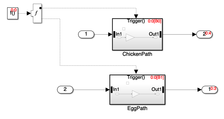
In the last example we showed that with independent data flows execution order is resolved by Simulink; however, there are instances where the execution order will matter (1). The “obvious” and very wrong solution is to add a data dependency to the path.

By adding a “Zero value gain” and sum block to the “Egg path” I have forced the “Chicken path” to be executed first (4). For reasons that should be obvious this is a bad idea. Anyone who looked at the model would think “Why are they doing that” and they would be correct in asking that question. The recommended approach is to make the execution order explicite using a Function driven approach

In this case the “Egg” is executing second; this is known from the “B” number in the block, “ChickenPath” is BO, while “EggPath” is B1; the lower number executes first. For more complex execution orders a Stateflow chart can be used to define the execution order

In this “tongue in beak” example we see that “eggs” only execute during the “WeHaveEggs” and the “Dinosaur” states. Once we hit the “WeHaveBoth” state (after many eons) the Chicken executes first. In my next post I will give examples of best practices for controlling execution order with Stateflow charts.

Footnotes:

1. Within the subsystem the execution order does not matter. However there are several cases where it can matter.
   1. Time limited execution: If the given function has a limited time for execution allocated and it is possible that all of the calculations may not be able to be performed in that time period. In that case you would want to control the execution order
   2. Consumption by parallel process: If the data from one (or more) of the paths is used by a parallel process and that process needs data “first” then you want to control the execution process.
   3. Determinism: For some analysis locking down execution order will simplify the execution task.
2. I debated even showing this image, however I have seen many “cleaver”(3) engineers come up with this solution.
3. Yeah, I realized I was autocorrected to “cleaver” as in something that cuts or chops . It was an error at first. Then I realized that I liked that more, they are not really “clever” rather they are just chopping apart a problem.
4. This could be considered a form of “playing chicken”

Please consider subscribing for regular email updates

Newton’s method is one of the foundational concepts in numerical mathematics; it is a method for finding the minimum value of real-valued functions through a series of successive approximations.  While the approach has limitations (it can be “trapped” in local minimum, it can be slow, …) it is the gateway algorithm(1).

Newton and Model-Based Design

Aside from the equations of motion, integration, theory of gravity (to start a long list) the children of Newton’s method are found in optimization problems. Optimization problems seek to find the minimize (or maximize) a value for a set of equations (or input data) based on the system input. Let’s consider an example of my Chevy Volt and optimizing energy use during my daily commute to work.

• Distance to work
• Range of battery
  • Effect of starting battery temperature
  • Driving conditions (highway / surface streets)
  • Cabin climate control (heating / cooling)
• Cost of
  • Charging the vehicle (at home / at work)
  • Gas (in the Volt the gas engine charges the battery)
• Externalities
  • Carbon emissions from the different energy sources.

When I frame this equation I set the commute as a “From-work-to-home-from-home-to-work” route. This, and thank you MathWorks, because there are free charging stations at my office, therefore any charging there is “free” (2).

• cost = C1 + C2 + C3
  • C1 = Cost_per_Kilowatt_Work * Charge + E1
    • C1 is at work co Cost_per_KW = 0 + E1 * Charge
  • C2 = Cost_per_Kilowatt_Home * Charge + E2
    • C2 = (0.12 + E2) * Charge
  • C3 = Cost_Per_Gallon * Gallons_Per_Kilowatt * Charge + E3
    • C3 = (3.50 * 30 + E3) * Charge

In this case the E1, E2 and E3 are the external costs for use of power. I don’t directly pay these costs(3) but from an ethical standpoint let us remember them.

The total charge is a function of distance, driving conditions and environmental conditions (do I run the heat or AC).

• Charge = F(Distance,DriveCond) + F(Cabin,Environment)

Skipping the analysis here to the conclusions. Since heating a car from the battery is very energy intensive, and since driving above 40 has a hit on fuel economy the “target” for short drives is to pre-heat the car (while at work) and to drive in a most sedate fashion. For medium drives the key is to use the engine heat the car and battery up at the start of the drive…

The “costs” of our decisions:

In the equations above there are “E” terms assigned to each of the costs, the “externalities” in economic terms. These “E” terms can be used to “weigh” the optimization function to push (or pull) the outcome towards a given solution. In some cases the value of the weights can be calculated, other times they are assigned based on a desired outcome. For example, if I was creating an optimization equation for the “ultimate chocolate bar” I would have a heavy penalty against coconut; there is nothing inherently wrong about coconut I just can’t stand it.

Integrating content in this post (4)

This post was written due to N simple observations

• Complex problems can be first understood using “base” methods: Real world optimization routines rarely used a Newton’s method due to efficiency issues, however for understanding optimization the simplicity of a Newton’s method can’t be beat.
• Concepts are Queen / King: The concept behind the Newton’s method, that successive approximations can lead to a numerical solution underpins multiple fields, optimization, feedback loops for controls, noise reduction…
• Reviewing “base” methods can lead to new understanding: In writing this post, and reviewing information on optimization and the basis of calculus (5) I have figured out solutions to a few problems that are plaguing me now, that of course will be in a future post

Footnotes

1. The gateway numerical method: Next thing you know you will be diving into implicit and explicate solutions to P.D.E.s
2. There is still an external cost for charging at work, that energy is produce somewhere so some amount of greenhouse gas is being produced. This sort of “local” or self optimization can be seen as a leading cause of global climate change.
3. This isn’t completely true, since I breath I do pay a direct cost to my health due to air pollution.
4. What post featuring Newton would be complete without integration
5. Calculus: from Latin, literally ‘small pebble’, with enough “small pebbles” you can “rock” the mathematical world.

If you find value in these posts, consider subscribing