The area under the curve, infinitesimally small slices, the integral is integral to control algorithms. With that in mind I wanted to point out a few “edge cases” in their use with in the Simulink environment.

Case 1: Standard execution

The standard execution would be inside of a continuously called subsystem. From calculus, remember that the integral of sine = cosine + C; which is what we see when we plot the results. So far so good.

Case 2: Execution context

Let’s look now at what happens when your execution context is not contiguous; in this case a conditionally called subsystem. In this case I will use an enabled subsystem to periodically call the integrator.

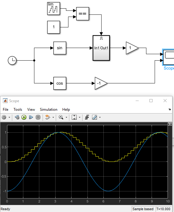
For this first example I reduced the sample rate by 50%. (E.g. the ramp function toggled between 0 and 1). As a result while the shape of the output is correct (a cosine) the amplitude is 1/2 the original value. I could correct by adding a gain factor on the output (or in the integral).

Note: when sampling data it is critical that the minimum sampling frequency is at least 2X faster than the frequency of the signal. This is know as the Nyquist Frequency

Case 3: Non-periodic

In some case sampling is event based. In this case it is critical that the events are more frequent than the Nyquist Frequency. However, since they cannot be assumed to be at a simple periodic frequency you cannot use a gain factor to correct for the sampling bias.

The simplest solution is to increase the frequency of the sample, the higher the frequency the more accurate the results.

Baring that a custom integrator can be applied that interpolates off of the last N data points and the temporal gaps; however this approach will not work if the temporal gaps are large or if the data is rapidly changing…

Case 4: Function called integrators

The final case to consider is when the integrator is part of a function call system. In most cases this will act like the periodic instance show above; there is however a special case, when the same function is called more than once in a single time step. In this instance only the first signal passed into the function will be “integrated”. Why?

Remember that integration can be expressed as a sum of slices multiplied by the time step. For the first call to the function the delta in time is the time step. For subsequent calls the time delta is zero.

If you need this functionality consider passing in the DT value as an external variable or performing the sum of two different function calls.

If you are enjoying these posts, please consider subscribing to them.