Every engineering project has a starting point where you map out what you want to realize and how you will enact your vision. For complicated projects there are iterations at each stage as the initial design process is honed in on and leads toward the final design. With this series of blog posts I am going to walk you through my design process for optimizing a set of my “historical daily commutes”(1) for fuel-efficiency.

The cost function

Optimization requires a function (or set of functions) to optimize against. Our first task then is to outline what will go into our “cost function.”(2)
- Vehicle physics
- Vehicle efficiency: engine & driveline
- Vehicle aerodynamics: the effect of speed on MPG
- Environmental factors
- Route topology: the ups and downs that make your MPG go up or down
- Weather: The rain, the sleet, and the snow that changes traction and heating you know…
- Human factors(3)
- Driver behavior: lead-footed devil or soft-coasting angel?
- Traffic conditions: what are the other drivers like?
Types of modeling

As I’ve written about before, one of the keys to creating a system is selecting the correct level of fidelity for your models. To that end I will consider:
- Vehicle physics: This can be done with basic “table lookup” models. Past experience shows that there are dimension returns on higher fidelity models/
- Environmental factors: The environment directly impacts the vehicle physics; modeling this can be done using real-world data (maps) and historical data (weather). These models will give us the chance to explore data-based modeling.
- Human factors: I will be drawing on network theory models for traffic flow and human/traffic interactions.
Optimizing the cost function

This is where things become interesting; this cost function is highly nonlinear. How we navigate (optimize) the cost function is an open question. I will try and consider which of the following is the best approach:
- Segmentation: decompose the optimization into sub-optimization problems and run integration analysis?
- Neural network: global optimization of the system?
- Model linearization: create a linearized version of the models enabling linear optimizations?
Footnote
- I will be selecting commuting routes from my early years of work when I was part of the auto industry. Travel to the GM Tech Center in Warren, Ford’s Scientific Research Labs, and the Milford Proving grounds. Each route will be analyzed individually and then the goodness-of-fit of the algorithm will be compared between the results.
- The objective with a cost function is to minimize the cost of the tasks. I’ve also seen this formulated as a “satisfaction quotient” where the objective is to maximize satisfaction. While I like the latter concept more, the minimization algorithms are simpler to implement so we will be using those.
- When driving in rush hour it can seem like you are the only human on the road until someone is nice and lets you merge over to that lane you’ve needed to for the past 10 minutes.


